Finite strain¶

Constitutive theory¶

For finite strain poromechanics, by writing Clausius-Duhem inequality (dissipation inequality) we can derive constitutive equations for solid and fluid phases as [ICR24] (see also (61) and discussion thereof)

(299)¶\[ \bm{S}^\rs_{E(\rs)} = 2\frac{\partial(\rho_{0(\rs)}^\rs\psi^\rs)}{ \partial \bm{C}_\rs}, \quad p_\rf = (\rho^{\fR})^2\frac{\partial \psi^\rf}{\partial \rho^{\fR}}, \]

where $\bm{S}^\rs_{E(\rs)}$ is effective second Piola-Kirchoff stress tensor, $\psi^\rs$ is strain energy per unit mass for the solid skeleton which is defined in previous sections for neo-Hookean model.

Helmholtz free energy per unit mass for fluid phase $\psi^\rf$ is given by

(300)¶\[ \psi^\rf = \frac{1}{2}\phi^\rf \bulk_\rf \left(\log \rho^{\fR}\right)^2, \]

which using second equation of (299), we arrive at constitutive equation for the real mass density of the pore fluid as

(301)¶\[ \rho^{\fR} = \rho^{\fR}_0 \exp\left( \frac{p_\rf - p_{\rf,0}}{\bulk_\rf}\right), \]

where $\rho^{\fR}_0, p_{\rf,0}$ are the initial real mass density and pore fluid pressure at time $t = 0$.

The total stress for the mixture for neo-Hookean model (83) (dropping now $(\cdot)_\rs$ subscripts where appropriate) is

(302)¶\[ \begin{aligned} \bm{S} &= J \bm{F}^{-1} \bm{\sigma} \bm{F}^{-T} = \bm{S}^\rs_E - J p_\rf \bm{C}^{-1}, \\ \bm{S}^\rs_E &= \firstlame_d J V' \bm{C}^{-1} + \secondlame_d \left( \bm{I} - \bm{C}^{-1} \right) = \frac{\firstlame_d}{2} \left( J^2 - 1 \right)\bm{C}^{-1} + \secondlame_d \left( \bm{I} - \bm{C}^{-1} \right), \end{aligned} \]

and using (25) we can write symmetric Kirchhoff stress tensor as

(303)¶\[ \begin{aligned} \bm{\tau} &= \bm{\tau}^\rs_E - J p_\rf \bm{I}, \\ \bm{\tau}^\rs_E &= \firstlame_d J V' \bm{I} + \secondlame_d \left( \bm{b} - \bm{I} \right) = \frac{\firstlame_d}{2} \left( J^2 - 1 \right)\bm{I} + \secondlame_d \left( \bm{b} - \bm{I} \right). \end{aligned} \]

Weak enforcement of solid incompressibility via strain-energy potential¶

For larger deformations, it is possible in the numerical sense to compute $J \leq \phi^{\rm{s}}_0$, which violates the solid incompressibility assumption (refer to (46)). [EE99] attempted to rectify this by modifying the neo-Hookean potential

(304)¶\[ \begin{aligned} V(J) := ({\rm{log}}(J))^2 \quad \text{or} \quad V(J) := \frac{1}{4}(J^2 - 1 - 2{\rm{log}}J) \end{aligned} \]

(305)¶\[ \begin{aligned} V(J) := (1 - \phi^\rs_0)^2\left(\frac{J - 1}{1 - \phi^\rs_0} - {\rm{log}}\left[\frac{J - \phi^\rs_0}{1 - \phi^\rs_0}\right]\right)\, . \end{aligned} \]

Then, the initial solid skeleton effective stress is

(306)¶\[ \begin{aligned} \bm{S}_E^\rs &= \firstlame(1 - \phi_0^\rs)^2 \left(\frac{J}{1 - \phi_0^\rs} - \frac{J}{J - \phi_0^\rs} \right)\bm{C}^{-1} + \secondlame \left( \bm{I} - \bm{C}^{-1} \right)\, , \end{aligned} \]

such that the solid skeleton effective stress in the current configuration is

(307)¶\[ \begin{aligned} \bm{\tau}_E^\rs &= \firstlame(1 - \phi_0^\rs)^2 \left(\frac{J}{1 - \phi_0^\rs} - \frac{J}{J - \phi_0^\rs} \right)\bm{I} + \secondlame \left(\bm{b} - \bm{I}\right)\, . \end{aligned} \]

Deformation-dependent porosity functions¶

Recall generalized Darcy’s law from (47):

\[ \dot{\bm{w}} = \phi^\rf\tilde{\bm{v}}_\rf = -\varkappa(\nabla_x p_\rf + \rho^\fR(\ddot{\bm{u}}_\rf - \bm{f}^\rf))\, , \]

where

\[ \varkappa = \frac{\varkappa_\circ}{\mu_\rf}\frac{\mathcal{F}(\phi^\rf)}{\mathcal{F}(\phi^\rf_0)}\, . \]

In addition to Kozeny-Carman (48), another suitable function was developed for soft tissues by [LMR81]:

\[ \mathcal{F}(\phi^\rf) = \exp[\kappa(J - 1)] = \exp\left[\kappa\left(\frac{\phi^\rs_0}{1 - \phi^\rf} - 1\right)\right]\, . \]

However, both the Kozeny-Carman and [LMR81] functional forms do not strictly satisfy the solid incompressibility constraint, which mandates a bound on the Jacobian of deformation: $\phi^\rs_0 < J < \infty$. This in turn mandates the behavior of $\mathcal{F}(\phi^\rf)$:

(311)¶\[ \begin{aligned} \mathcal{F}(\phi^\rf) \rightarrow \begin{Bmatrix}0 \\ 1\end{Bmatrix} \text{ if } \begin{cases} \phi^\rf \rightarrow 0 \Leftrightarrow \phi^\rs \rightarrow 1 \Leftrightarrow J \rightarrow \phi_0^\rs\\ \phi^\rf \rightarrow 1 \Leftrightarrow \phi^\rs \rightarrow 0 \Leftrightarrow J \rightarrow \infty\end{cases}\, , \end{aligned} \]

in other words, for vanishing porosity we should obtain a solid-like material and for full porosity (fully expanded solid) the solid-fluid interactions should be negligible beyond the viscous drag forces induced by $\varkappa_\circ/\mu_\rf$.

As such, [Eip98] proposed a deformation dependent permeability that respects the restriction of materially incompressible solid constituent:

\[ \begin{aligned} \mathcal{F}(\phi^\rf) = (\phi^\rf)^\kappa \end{aligned} \]

for $\kappa > 0$, however, such a function is ill-suited for rapidly expanding materials (see A comparison, adapted from Markert2005, of different deformation-dependent hydraulic conductivities for \kappa = 3.0 (a) showing the instability of the Kozeny-Carman relation for high compression of the drained mixutre (solid skeleton) and (b) a zoomed-in version of (a) showing the inadequacy of the Eipper1998 model for high expansion of the drained mixture (solid skeleton).). In light of this, [Mar05] proposed

\[ \begin{aligned} \mathcal{F}(\phi^\rf) = \Bigg(\frac{\phi^\rf}{1 - \phi^\rf}\Bigg)^\kappa \, , \end{aligned} \]

such that

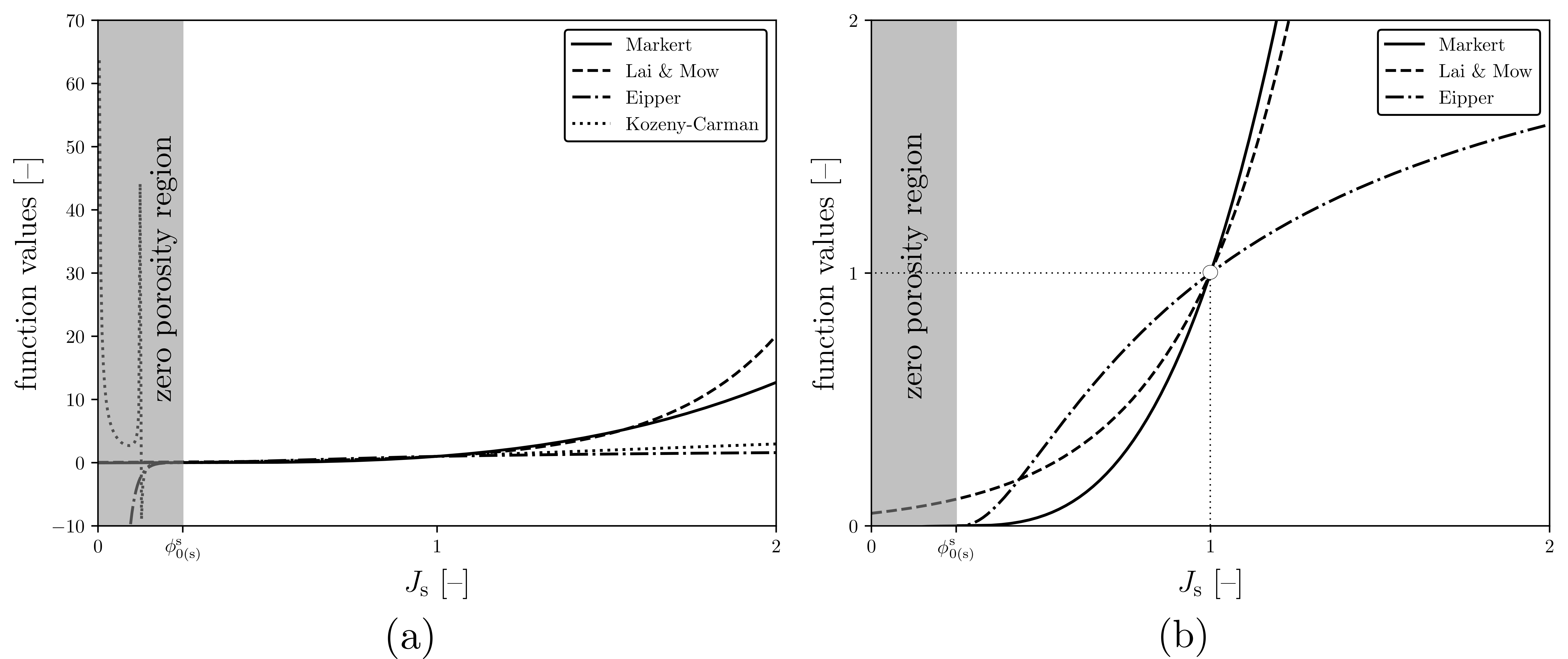
\[ \begin{aligned} \varkappa = \frac{\varkappa_{\circ}}{\mu_\rf}\Bigg(\frac{J - \phi_0^\rs}{1 - \phi_0^\rs}\Bigg)^\kappa\, . \end{aligned} \]

../../../../../_images/permeability-functionals.png — Fig. 6 A comparison, adapted from [Mar05], of different deformation-dependent hydraulic conductivities for $\kappa = 3.0$ (a) showing the instability of the Kozeny-Carman relation for high compression of the drained mixutre (solid skeleton) and (b) a zoomed-in version of (a) showing the inadequacy of the [Eip98] model for high expansion of the drained mixture (solid skeleton).¶

Isentropic ideal gas pore fluid¶

So far, we have assumed an exponential model for the barotropic pore fluid model where $\bulk_\rf$ denoted an isentropic bulk modulus. When the pore fluid is an ideal gas, then at larger pore fluid pressures such a model is ill-suited for describing the pore fluid (gas) deformation when compared to the Hugoniot in the absence of solid-fluid coupling (see figure below where compression is defined as $1 - J_\rf$). A more appropriate constitutive model is that of an isentropic ideal gas:

(312)¶\[ \rho^\fR = \rho^\fR_0\left(\frac{p_\rf}{p_{\rf,0}}\right)^{1/\Gamma}\, , \]

where the ratio of specific heats $\Gamma := c_p/c_v$ and $c_p$ and $c_v$ are constant specific heats of the pore fluid at constant pressure and constant volume, respectively. For example, for air $\Gamma = 1.4$.

Click to show code

import numpy as np
import pandas as pd
import altair as alt

# Constants
p0     = 101.325e3
G      = 1.4
Keta   = G * p0
Ktheta = p0

# Generate data
J = np.linspace(1, 0.3, 50)

df = pd.DataFrame({
    'J': J,
    '1_minus_J': 1 - J,
    'Hugoniot ideal gas': p0 * ((G + 1) - (G - 1) * J) / ((G + 1) * J - (G - 1)),
    'isentropic ideal gas': p0 * (J ** (-G)),
    'isothermal ideal gas': p0 / J,
    'isentropic exp.': p0 - Keta * np.log(J),
    'isothermal exp.': p0 - Ktheta * np.log(J)
})

# Convert to kPa and offset
for col in df.columns[2:]:
    df[col] = df[col] * 1e-3 - 101.325

# Melt to long format for Altair
df_long = df.melt(id_vars=['1_minus_J'], value_vars=df.columns[2:],
                  var_name='curve', value_name='p')

# Filter out out-of-bounds points (Altair doesn't always clip)
df_long = df_long[(df_long['p'] >= 0) & (df_long['p'] <= 200)]

# Add dash style
df_long['dash'] = df_long['curve'].apply(
    lambda x: 'dashed' if x == 'isentropic ideal gas' else 'solid'
)

# Plot
alt.Chart(df_long).mark_line(clip=True).encode(
    x=alt.X('p:Q', title='Overpressure [kPa]', scale=alt.Scale(domain=[0, 200])),
    y=alt.Y('1_minus_J:Q', title='Pore fluid compression', scale=alt.Scale(domain=[0.0, 0.65])),
    color=alt.Color('curve:N', title='Model'),
    strokeDash=alt.StrokeDash('dash:N', legend=None)
)

This of course alters the balance of mass of the pore fluid since the material time derivative of the pore fluid real mass density is now

\[ \frac{D^\rf \rho^\fR}{Dt} = \frac{\rho^\fR_0}{\Gamma p_\rf}\left(\frac{p_\rf}{p_{\rf,0}}\right)^{1/\Gamma}\frac{D^\rf p_\rf}{Dt} = \frac{\rho^\fR}{\Gamma p_\rf}\frac{D^\rf p_\rf}{Dt}\, , \]

where the change from the exponential barotropic model is $\Gamma p_\rf$ in place of $\bulk_\rf$. Thus the balance of mass of the mixture may be written in the current configuration as

(313)¶\[ \frac{\phi^\rf}{\Gamma p_\rf}\frac{D p_\rf}{D t} + \nabla_x\cdot\dot{\bm{u}} + \nabla_x\cdot\dot{\bm w} + \frac{\dot{\bm w}}{\Gamma p_\rf} \cdot \nabla_x p_\rf = \frac{\hat{\rho}^{\rf}}{\rho^{\fR}}. \]

Strong and weak formulations¶

To derive the strong form for finite strain poromechanics, we use the balance of momentum of the mixture (54)$_1$ (under the assumption that $\ddot{\bm{u}} = \bm{0}$) and balance of mass of the mixture (44) as

(314)¶\[ \begin{aligned} -\nabla_X \cdot \bm{P} - \rho_0 \bm g &= 0, \qquad \text{in $\Omega_0$} \\ \frac{\phi^\rf}{\bulk_\rf}\frac{D p_\rf}{D t} + \nabla_x\cdot \dot{\bm{u}} + \nabla_x\cdot \dot{\bm w} + \frac{\dot{\bm w}}{\bulk_\rf}\cdot \nabla_x p_\rf &= 0, \qquad \text{in $\Omega$} \\ \bm{u} &= \bar{\bm u}, \quad \text{on $\partial \Omega^{D}_0$} \\ p_\rf &= \bar{p}_\rf, \quad \text{on $\partial \Omega^{D}$} \\ \bm{P} \cdot \bm N &= \bar{\bm t}, \qquad \text{on $\partial \Omega^{N}_0$} \\ \dot{\bm{w}} \cdot \bm n &= \bar{s}, \qquad \text{on $\partial \Omega^{N}$} \\ \bm u &= \bm u_0, \qquad \text{in $\Omega_0$} \\ p_\rf &= p_{\rf,0}, \qquad \text{in $\Omega$} \end{aligned} \]

where we have dropped subscript $(\cdot)_\rs$ by convention, $\bm N$ and $\bm n$ are the unit normal vectors on the face in initial and current configurations, $_X$ and $_x$ in $\nabla_X, \nabla_x$ indicate that the gradient are calculated with respect to the initial/current configurations. Multiplying the strong form (314) by test functions $(\bm{v}, q)$ and integrate by parts, we can obtain the weak form for finite strain hyperporoelasticity as: find $(\bm{u}, p_\rf) \in \mathcal{V} \times \mathcal{Q} \subset H^1 \left( \Omega_0 \right) \times H^1 \left( \Omega_0 \right)$ such that

(315)¶\[ \begin{aligned} r_u(\bm u, p_\rf) &\coloneqq \int_{\Omega_0}{\nabla_x \bm{v} \tcolon \bm{\tau}} \, dV - \int_{\Omega_0}{\bm{v} \cdot \rho_0 \bm{g}} \, dV - \int_{\partial \Omega_0}{\bm{v} \cdot \bar{\bm t}} \, dA = 0, \quad \forall \bm{v} \in \mathcal{V}, \\ r_{p_\rf}(\bm u, p_\rf) &\coloneqq \int_{\Omega_0} q \cdot \left( \frac{\phi^\rf}{\bulk_\rf}\dot{p}_\rf + \nabla_x\cdot \dot{\bm{u}} - \frac{\varkappa}{\bulk_\rf}\nabla_x p_\rf \cdot \nabla_x p_\rf \right) J \, dV \\ &+\int_{\Omega_0} \nabla_x q \cdot \varkappa \nabla_x p_\rf \, J dV + \int_{\partial \Omega}{ q \, \bar{s}} \, da = 0, \quad \forall q\in \mathcal{Q}, \\ \end{aligned} \]

where we have used the push forward (103) to write the first equation with respect to $_x$ and $\bm \tau$, and replaced $\dot{\bm w} = -\varkappa \nabla_x p_\rf$ by assuming $\ddot{\bm u} = \bm{0}$ and $\bm f^\rf = \bm{0}$ in (49), the latter of which implies that $\bm{g} = \bm{0}$. The definition for $\bm{\tau}$ for the standard neo-Hookean model for the drained mixture (solid skeleton) response is given in (303).

For the isentropic ideal gas model (Isentropic ideal gas pore fluid), we have for the strong form

(316)¶\[ \begin{aligned} -\nabla_X \cdot \bm{P} - \rho_0 \bm g &= 0, \qquad \text{in $\Omega_0$} \\ \frac{\phi^\rf}{\Gamma p_\rf}\frac{D p_\rf}{D t} + \nabla_x\cdot \dot{\bm{u}} + \nabla_x\cdot \dot{\bm w} + \frac{\dot{\bm w}}{\Gamma p_\rf}\cdot \nabla_x p_\rf &= 0, \qquad \text{in $\Omega$} \\ \bm{u} &= \bar{\bm u}, \quad \text{on $\partial \Omega^{D}_0$} \\ p_\rf &= \bar{p}_\rf, \quad \text{on $\partial \Omega^{D}$} \\ \bm{P} \cdot \bm N &= \bar{\bm t}, \qquad \text{on $\partial \Omega^{N}_0$} \\ \dot{\bm{w}} \cdot \bm n &= \bar{s}, \qquad \text{on $\partial \Omega^{N}$} \\ \bm u &= \bm u_0, \qquad \text{in $\Omega_0$} \\ p_\rf &= p_{\rf,0}, \qquad \text{in $\Omega$} \end{aligned} \]

and for the weak form

(317)¶\[ \begin{aligned} r_u(\bm u, p_\rf) &\coloneqq \int_{\Omega_0}{\nabla_x \bm{v} \tcolon \bm{\tau}} \, dV - \int_{\Omega_0}{\bm{v} \cdot \rho_0 \bm{g}} \, dV - \int_{\partial \Omega_0}{\bm{v} \cdot \bar{\bm t}} \, dA = 0, \quad \forall \bm{v} \in \mathcal{V}, \\ r_{p_\rf}(\bm u, p_\rf) &\coloneqq \int_{\Omega_0} q \cdot \left( \frac{\phi^\rf}{\Gamma p_\rf}\dot{p}_\rf + \nabla_x\cdot \dot{\bm{u}} - \frac{\varkappa}{\Gamma p_\rf}\nabla_x p_\rf \cdot \nabla_x p_\rf \right) J \, dV \\ &+\int_{\Omega_0} \nabla_x q \cdot \varkappa \nabla_x p_\rf \, J dV + \int_{\partial \Omega}{ q \, \bar{s}} \, da = 0, \quad \forall q\in \mathcal{Q}, \\ \end{aligned} \]

Linearization¶

As explained in Linearization: initial configuration, we need the Jacobian form of the (315) which is: find $(\diff \bm{u}, \diff p_\rf) \in \mathcal{V} \times \mathcal{Q}$ such that

(318)¶\[ \begin{aligned} &\int_{\Omega_0} \nabla_x \bm{v} \tcolon \left( \diff \bm{\tau} -\bm{\tau}(\nabla_x \diff\bm{u})^T \right) dV = -r_u, \quad \forall \bm{v} \in \mathcal{V}, \\ &\int_{\Omega_0} q \, \left( \diff L J + L \diff J \right) dV + \int_{\Omega_0} \nabla_x q \cdot (\diff K - K\nabla_x\diff\bm{u})\, dV = -r_{p_\rf}, \quad \forall q \in \mathcal{Q} \end{aligned} \]

where

\[ \begin{aligned} \diff \bm{\tau} -\bm{\tau}(\nabla_x \diff\bm{u})^T &= \diff \bm{\tau}_E^\rs -\bm{\tau}_E^\rs(\nabla_x \diff\bm{u})^T - \left(\diff J p_\rf + J \diff p_\rf \right) \bm I + J p_\rf (\nabla_x \diff\bm{u})^T, \\ &= (\nabla_x \diff\bm{u}) \bm{\tau} + \bm{F} \diff \bm{S}_E^\rs \bm{F}^T - \left(\diff J p_\rf + J \diff p_\rf \right) \bm I + 2 J p_\rf \diff\bm\epsilon, \\ L &= \frac{\phi^\rf}{\bulk_\rf}\dot{p}_\rf + \nabla_x\cdot \dot{\bm{u}} - \frac{\varkappa}{\bulk_\rf}\nabla_x p_\rf \cdot \nabla_x p_\rf, \\ \diff L &= \mathrm{shift_v} \left(\frac{\phi^\rf}{\bulk_\rf}\diff p_\rf + \diff \, \left(\nabla_x\cdot \bm{u} \right) \right) - \frac{\diff \varkappa}{\bulk_\rf}\nabla_x p_\rf \cdot \nabla_x p_\rf - 2 \frac{\varkappa}{\bulk_\rf}\nabla_x p_\rf \cdot \diff \, (\nabla_x p_\rf), \\ K &= \varkappa \nabla_x p_\rf J\, ,\\ \diff K &= \diff \varkappa \nabla_x p_\rf \, J + \varkappa \diff \, (\nabla_x p_\rf) \, J + \varkappa \nabla_x p_\rf \diff J, \end{aligned} \]

with given $\diff \bm{\tau}_E^\rs -\bm{\tau}_E^\rs(\nabla_x \diff\bm{u})^T$ in (111) for example with the standard neo-Hookean model and

\[ \begin{aligned} \diff J &= J \, \trace (\nabla_x \diff\bm u) = J \, \trace \diff\bm\epsilon, \\ \diff \varkappa &= \frac{\varkappa_{\circ}}{\mu_\rf \mathcal{F}(\phi^\rf_0)} \diff \mathcal{F}(\phi^\rf) = \frac{\varkappa_{\circ}}{\mu_\rf \mathcal{F}(\phi^\rf_0)} \frac{\partial \mathcal{F}(\phi^\rf)}{\partial \phi^\rf} \diff \phi^\rf = \varkappa\frac{\partial\mathcal{F}(\phi^\rf)}{\partial\phi^\rf} \mathcal{F}(\phi^\rf)^{-1} \diff \phi^\rf, \\ \diff \phi^\rf &= \diff \left(1 - \phi^\rs \right) = \diff \left(1 - \frac{\phi^\rs_0}{J} \right) = \frac{\phi^\rs_0}{J^2} \diff J = \phi^\rs \trace \diff\bm\epsilon, \\ \diff \, (\nabla_x p_\rf) &= \diff \, \left( \bm{F}^{-T} \nabla_X p_\rf \right) = \nabla_x \diff p_\rf - (\nabla_x \diff\bm{u})^T \nabla_x p_\rf, \\ \diff \, \left(\nabla_x \cdot \bm{u} \right) &= \diff \, \trace \left( \nabla_x \bm{u}\right) = \diff \, \trace \left( \nabla_X \bm{u} \bm{F}^{-1}\right) = \trace \left( \nabla_x \diff \bm{u} - \nabla_x \bm{u} \nabla_x \diff \bm{u}\right), \\ &= \nabla_x \cdot \diff\bm{u} - \nabla_x \bm{u} \tcolon (\nabla_x \diff\bm{u})^T, \end{aligned} \]

where $\mathcal{F}(\phi^\rf)$ is defined, for example, in (48).

For the isentropic ideal gas model (Isentropic ideal gas pore fluid), the mixture mass balance terms are different from the exponential model such that the following term is used in place of $L$ above:

\[ \begin{aligned} L &= \frac{\phi^\rf}{\Gamma p_\rf}\dot{p}_\rf + \nabla_x\cdot \dot{\bm{u}} - \frac{\varkappa}{\Gamma p_\rf}\nabla_x p_\rf \cdot \nabla_x p_\rf, \\ \diff L &= \mathrm{shift_v} \left(\frac{\phi^\rf}{\Gamma p_\rf}\diff p_\rf + \diff \, \left(\nabla_x\cdot \bm{u} \right) \right) - \frac{\phi^\rf}{\Gamma (p_\rf)^2}\dot{p}_\rf \diff p_\rf\\ &\phantom{=} - \frac{\diff \varkappa}{\Gamma p_\rf}\nabla_x p_\rf \cdot \nabla_x p_\rf - 2 \frac{\varkappa}{\bulk_\rf}\nabla_x p_\rf \cdot \diff \, (\nabla_x p_\rf) + \frac{\varkappa}{\Gamma (p_\rf)^2}\nabla_x p_\rf \cdot \nabla_x p_\rf \diff p_\rf\, . \end{aligned} \]

Generic weak formulation¶

For overview on generic weak form implementation for the poromechanics model, see Generic weak formulation. Here we define

\[ \begin{aligned} \bm f_0 &= -\rho_0 \bm g = \bm{0}, \quad \bm f_1 = \bm{\tau} = \bm{\tau}_E^\rs - J p_\rf \bm{I}, \\ \bm g_0 &= L \, J = \left( \frac{\phi^\rf}{\bulk_\rf}\dot{p}_\rf + \nabla_x\cdot \dot{\bm{u}} - \frac{\varkappa}{\bulk_\rf}\nabla_x p_\rf \cdot \nabla_x p_\rf \right) J, \quad \bm g_1 = K = \varkappa \nabla_x p_\rf \, J, \\ \diff \bm f_1 &= \diff \bm{\tau} -\bm{\tau}(\nabla_x \diff\bm{u})^T, \quad \diff \bm g_0 = \diff L J + L \diff J, \\ \diff \bm g_1 &= \diff K - K\nabla_x\diff \bm{u} = \diff \varkappa \nabla_x p_\rf \, J + \varkappa \diff \, (\nabla_x p_\rf) \, J + \varkappa \nabla_x p_\rf \diff J - \varkappa \nabla_x p_\rf J\nabla_x \diff \bm{u} . \end{aligned} \]

Note that, technically speaking, $\bm f_0$ needs to be linearized under the assmption of $\bm{g} \neq \bm{0}$ (and by extension $\bm{f}^\rf \neq \bm{0}$) in the case of evolving volume fractions and/or compressible pore fluid. However, at this time, we continue to assume the body force acting on the mixture to be zero.

For dynamic example acceleration is not zero and we use the PETSc Timestepper (TS) object to manage timestepping. Specifically, Ratel uses the Generalized-Alpha method for second order systems (TSALPHA2) to solve the second order system of equations. More information on the PETSc TSALPHA2 time stepper can be found in the PETSc documentation TS.

We add

(319)¶\[ \begin{aligned} &\int_{\Omega_0} \bm v \cdot \left(\rho^b_0 \, \ddot{\bm u} \right) \, dV = \int_{\Omega_0} \bm v \cdot \left(J \rho^b \, \ddot{\bm u} \right) \, dV, \\ &\int_{\Omega_0} q \left(-\varkappa \, \ddot{\bm u} \cdot \nabla_x p_\rf\right) \frac{J \, \rho^{\fR}}{\bulk_\rf} dV + \int_{\Omega_0} \nabla_x q \cdot \left(\varkappa \rho^{\fR} J \, \ddot{\bm u}\right) \, dV, \end{aligned} \]

to the first and second equations of (315), such that

\[ \begin{aligned} \bm f_0 &\mathrel{+}= J\rho^b\ddot{\bm{u}}\, ,\\ \bm g_0 &\mathrel{+}= -\frac{\varkappa}{\bulk_\rf}\nabla_x p_\rf\cdot(\rho^\fR\ddot{\bm{u}})J\,\\ \bm g_1 &\mathrel{+}= \varkappa\rho^\fR\ddot{\bm{u}} J\, , \end{aligned} \]

and the jacobian is

(320)¶\[ \begin{aligned} &\int_{\Omega_0} \bm v \cdot \left(\diff J \rho^b \, \ddot{\bm u} + J \diff \rho^b \, \ddot{\bm u} + J \rho^b \, \mathrm{shift_a} \, \diff \bm u \right) \, dV, \\ &\int_{\Omega_0} q \left[-\diff \varkappa \, \ddot{\bm u} \cdot \nabla_x p_\rf - \varkappa \, \mathrm{shift_a} \diff \bm u \cdot \nabla_x p_\rf - \varkappa \, \ddot{\bm u} \cdot \diff \left(\nabla_x p_\rf \right) \right] \frac{J \, \rho^{\fR}}{\bulk_\rf} dV \\ &\int_{\Omega_0} q \left(-\varkappa \, \ddot{\bm u} \cdot \nabla_x p_\rf\right) \frac{\left(\diff J \rho^{\fR} + J \, \diff \rho^{\fR}\right)}{\bulk_\rf} \, dV + \\ &\int_{\Omega_0} \nabla_x q \cdot \left[ \left(\diff \varkappa \rho^{\fR} J + \varkappa \diff \rho^{\fR} J + \varkappa \rho^{\fR} \diff J \right) \ddot{\bm u} + \varkappa \rho^{\fR} J \, \mathrm{shift_a}\diff \bm u - \varkappa \rho^{\fR} J (\nabla_x \diff \bm u) \ddot{\bm u} \right] \, dV, \end{aligned} \]

such that,

\[ \begin{aligned} \diff \bm f_0 &\mathrel{+}= \diff J \rho^b \, \ddot{\bm u} + J \diff \rho^b \, \ddot{\bm u} + J \rho^b \, \mathrm{shift_a} \, \diff \bm u\, ,\\ \diff \bm g_0 &\mathrel{+}= \left[-\diff \varkappa \, \ddot{\bm u} \cdot \nabla_x p_\rf - \varkappa \, \mathrm{shift_a} \diff \bm u \cdot \nabla_x p_\rf - \varkappa \, \ddot{\bm u} \cdot \diff \left(\nabla_x p_\rf \right) \right] \frac{J \, \rho^{\fR}}{\bulk_\rf}\\ &\phantom{\mathrel{+}=} + \left(-\varkappa \, \ddot{\bm u} \cdot \nabla_x p_\rf\right) \frac{\left(\diff J \rho^{\fR} + J \, \diff \rho^{\fR}\right)}{\bulk_\rf}, \\ \diff \bm g_1 &\mathrel{+}= \left(\diff \varkappa \rho^{\fR} J + \varkappa \diff \rho^{\fR} J + \varkappa \rho^{\fR} \diff J \right) \ddot{\bm u} + \varkappa \rho^{\fR} J \, \mathrm{shift_a}\diff \bm u - \varkappa \rho^{\fR} J (\nabla_x \diff \bm u) \ddot{\bm u}\, , \end{aligned} \]

where using (301) we have

\[ \begin{aligned} \diff \rho^b &= \left(\rho^{\fR}-\rho^{\sR} \right) \diff \phi^\rf + \phi^\rf \diff \rho^{\fR}, \\ \diff \rho^{\fR} &= \frac{\rho^{\fR}_0 \, \diff p_\rf}{\bulk_\rf} \exp\left( \frac{p_\rf - p_{\rf,0}}{\bulk_\rf}\right) = \frac{\diff p_\rf}{\bulk_\rf}\rho^{\fR}. \end{aligned} \]

Note that unlike linear case where the porosity and density are constant, in finite strain we have assumed that the real mass density of the pore fluid is a function of pore fluid pressure (real mass density of solid is assumed constant, see (45)). Therefore, we use the mixture density in the current configuration $\rho^b$ in residual and jacobian to account for its variation with respect to pore fluid pressure.

For the isentropic ideal gas model (Isentropic ideal gas pore fluid), the mixture mass balance terms are different from the exponential model such that the following

(321)¶\[ \begin{aligned} &\int_{\Omega_0} q \left(-\varkappa \, \ddot{\bm u} \cdot \nabla_x p_\rf\right) \frac{J \, \rho^{\fR}}{\Gamma p_\rf} dV, \end{aligned} \]

is added to the second equation of (317), such that

\[ \begin{aligned} \bm g_0 &\mathrel{+}= -\frac{\varkappa}{\Gamma p_\rf}\nabla_x p_\rf\cdot(\rho^\fR\ddot{\bm{u}})J\, , \end{aligned} \]

and the jacobian is

(322)¶\[ \begin{aligned} &\int_{\Omega_0} q \left[-\diff \varkappa \, \ddot{\bm u} \cdot \nabla_x p_\rf - \varkappa \, \mathrm{shift_a} \diff \bm u \cdot \nabla_x p_\rf - \varkappa \, \ddot{\bm u} \cdot \diff \left(\nabla_x p_\rf \right) \right] \frac{J \, \rho^{\fR}}{\Gamma p_\rf} dV + \\ &\int_{\Omega_0} q \left(-\varkappa \, \ddot{\bm u} \cdot \nabla_x p_\rf\right) \frac{\left(\diff J \rho^{\fR} + J \, \diff \rho^{\fR}\right)}{\Gamma p_\rf} \, dV + \\ &\int_{\Omega_0} -q \left(-\varkappa \, \ddot{\bm u} \cdot \nabla_x p_\rf\right) \frac{J \rho^{\fR}}{\Gamma (p_\rf)^2}\diff p_\rf \, dV\, , \end{aligned} \]

such that

\[ \begin{aligned} \diff \bm g_0 &\mathrel{+}= \left[-\diff \varkappa \, \ddot{\bm u} \cdot \nabla_x p_\rf - \varkappa \, \mathrm{shift_a} \diff \bm u \cdot \nabla_x p_\rf - \varkappa \, \ddot{\bm u} \cdot \diff \left(\nabla_x p_\rf \right) \right] \frac{J \, \rho^{\fR}}{\Gamma p_\rf}\\ &\phantom{\mathrel{+}=} + \left(-\varkappa \, \ddot{\bm u} \cdot \nabla_x p_\rf\right) \frac{\left(\diff J \rho^{\fR} + J \, \diff \rho^{\fR}\right)}{\Gamma p_\rf} - \left(-\varkappa\, \ddot{\bm u} \cdot \nabla_x p_\rf\right) \frac{J\rho^\fR}{\Gamma (p_\rf)^2}\diff p_\rf, \\ \end{aligned} \]

where using (312) we have

\[ \diff \rho^\fR = \frac{\rho^\fR}{\Gamma p_\rf} \diff p_\rf \, . \]

Pore fluid pressure stabilization¶

For stabilizing equal order elements, we follow the approach of [TZ06], which is based on the method of [BPitkaranta84]. The stabilization term acts like an opposing pore fluid pressure flux in the weak formulation of the balance of mass of the mixture (e.g., assuming exponential model for barotropic pore fluid, but extensible to any pore fluid constitutive model), such that

\[ \begin{aligned} r_{p_\rf}(\bm u, p_\rf) &\coloneqq \int_{\Omega_0} q \cdot \left( \frac{\phi^\rf}{\bulk_\rf}\dot{p}_\rf + \nabla_x\cdot \dot{\bm{u}} - \frac{\varkappa}{\bulk_\rf}\nabla_x p_\rf \cdot \nabla_x p_\rf \right) J \, dV \\ &+\int_{\Omega_0} \nabla_x q \cdot \left(\varkappa \nabla_x p_\rf + {\color{red}\alpha^\text{stab}\nabla_x\dot{p}_\rf}\right)\, J dV + \int_{\partial \Omega}{ q \, \bar{s}} \, da = 0, \quad \forall q\in \mathcal{Q}, \\ \end{aligned} \]

where the stabilization term is shown in red (and may also be enabled for dynamic cases). While [TZ06] have been able to relate the pressure stabilization parameter $\alpha^\text{stab}$ (units m$^3$-s$^2$/kg) to material geometry and simulation time-step, such an approach would be difficult to derive for compressible pore fluid and large deformations. Therefore, we choose $\alpha^\text{stab}$ on an ad-hoc basis. For incompressible pore fluid (i.e., $\bulk_\rf \sim $ GPa), choosing larger values $\mathcal{O}(10^{-6})$ tends to provide decent stability as compared to smaller values. For more compressible pore fluid (i.e., lower $\bulk_\rf \sim$ kPa) choosing smaller values $\mathcal{O}(10^{-10})$ tends to provide decent stability as compared to larger values.

For generic weak formulation, two additional terms are present for $\bm{g}_1$ and $\diff\bm{g}_1$, such that

\[ \begin{aligned} \bm g_1 &\mathrel{+}= J\alpha^\text{stab}\nabla_x\dot{p}_\rf\, ,\\ \diff \bm g_1 &\mathrel{+}= \alpha^\text{stab}\left(\diff J \, \nabla_x\dot{p}_\rf + J \mathrm{shift_v} \diff(\nabla_x p_\rf) - J\nabla_x\dot{p}_\rf(\nabla_x \diff \bm u)\right)\, . \end{aligned} \]

Note that pressure stabilization can be added to unequal order elements as well. In [IRC23] it was shown that under conditions of 1-D uniaxial strain, pressure stabilization improved computational performance for Hermite cubic-Lagrange linear displacement-pressure elements.

Command-line interface¶

To enable the finite strain, neo-Hookean-based poromechanics model, use the model option -model poromechanics-neo-hookean and set the material parameters listed in Finite strain poromechanics model options. Any parameter without a default option is required.

Table 34 Finite strain poromechanics model options¶
Option	Description	Default Value
`-model poromechanics-neo-hookean-current`	Required to enable the finite strain poromechanics model.
`-lambda_d [real]`	First Lame parameter for drained mixture (solid skeleton), $\lambda_d >= 0$
`-mu_d [real]`	Shear modulus for drained mixture (solid skeleton), $\mu_d >= 0$
`-bulk_d [real]`	Bulk modulus for drained mixture (solid skeleton), $\bulk_d >= 0$
`-bulk_s [real]`	Bulk modulus for solid, $\bulk_\rs >= 0$
`-bulk_f [real]`	Bulk modulus for pore fluid, $\bulk_\rf >= 0$
`-rho [real]`	Real solid mass density, $\rho^\sR_0 > 0$	`1.0`
`-rho_fR0 [real]`	Real pore fluid mass density, $\rho^\fR_0 > 0$	`1.0`
`-phi [real]`	Porosity, $0 < \phi^\rf < 1$
`-mu_f [real]`	Pore fluid viscosity, $\mu_\rf >= 0$
`-varkappa_0 [real]`	Intrinsic permeability, $\varkappa_{0} >= 0$
`alpha_stab [real]`	Pore fluid pressure stabilization, $\alpha^\text{stab} > 0$	`0.0` (default: disabled)
`-kappa [real]`	Hyperbolic porosity model exponent, $\kappa >= 0$	`-1.0` (default: Kozeny-Carman model)
`-Gamma [real]`	Ideal gas ratio of specific heats, $\Gamma > 0$	`0.0` (default: exponential model)
`-pf_0 [real]`	Initial pore fluid pressure (required $> 0$ when $\Gamma > 0$)	`0.0`

Note that when -pf_0 is set to a non-zero value, we also require the user supply a non-zero initial condition and the pressure boundary condition on the traction load face(s) (if applicable), e.g.,

ic:
  non_zero: 0., pf_0

bc:
  pressure: [facenumber]
  pressure_[facenumber]: pf_0
  pressure_[facenumber]_times: 0.

where pf_0 will be replaced by a [real] value corresponding to the -pf_0 option.

An example using the finite strain poromechanics model can be run via

$ ./bin/ratel-dynamic -options_file examples/ymls/ex03-dynamic-poromechanics-neo-hookean-current-pstab-pcfieldsplit-lu.yml