Material point method¶

Overview¶

The Material Point Method (MPM) is a numerical technique particularly well-suited for problems involving large deformations, history-dependent materials, and complex interactions such as contact and fracture. Originally developed as an extension of the FLIP method, MPM combines the advantages of Lagrangian and Eulerian approaches by tracking material points (particles) through a fixed background grid. This hybrid formulation enables the method to bypass mesh entanglement issues that plague conventional Lagrangian finite element methods during severe deformation scenarios. One way to summarise the material point method is: a finite element method where the integration points (material points) are allowed to move independently of the mesh [CAB+20b].

In MPM, state variables such as mass, momentum, and stress are carried by the particles, while a background mesh is used temporarily at each time step to solve the governing equations. This decoupling allows efficient simulation of a wide range of materials including elasto-plastic solids, granular media, and viscoelastic fluids. Explicit time integration schemes are commonly used for their simplicity, though recent developments have introduced robust implicit formulations that offer improved stability and larger time steps for quasi-static and dynamic applications.

Weak formulations¶

Large deformation analysis in Lagrangian mechanics typically follows either a total or updated formulation, distinguished by the frame in which equilibrium is applied. The total Lagrangian approach enforces equilibrium in the initial (undeformed) configuration, while the updated Lagrangian approach does so in the current (deformed) state. Fig. 8 (copied from [CAB+20b]) shows how a material point moves from its original position \(X_i\) to a previous converged position \(\tilde{X}_i\) and finally to the current deformed position \(x_i\), with an incremental deformation \(\Delta F_{ij}=\tilde{F}_{ij}\). As the point convects through the background mesh (original mesh in solid lines, deformed mesh in dashed lines), its local position change, potentially crossing into new elements.

In material point methods (MPM), the mesh is reset after each step, leading to a loss of information between configurations and making the updated formulation more natural fit, since mapping derivatives back to the reference frame—as needed in a total formulation—would be cumbersome [CAB+20b].

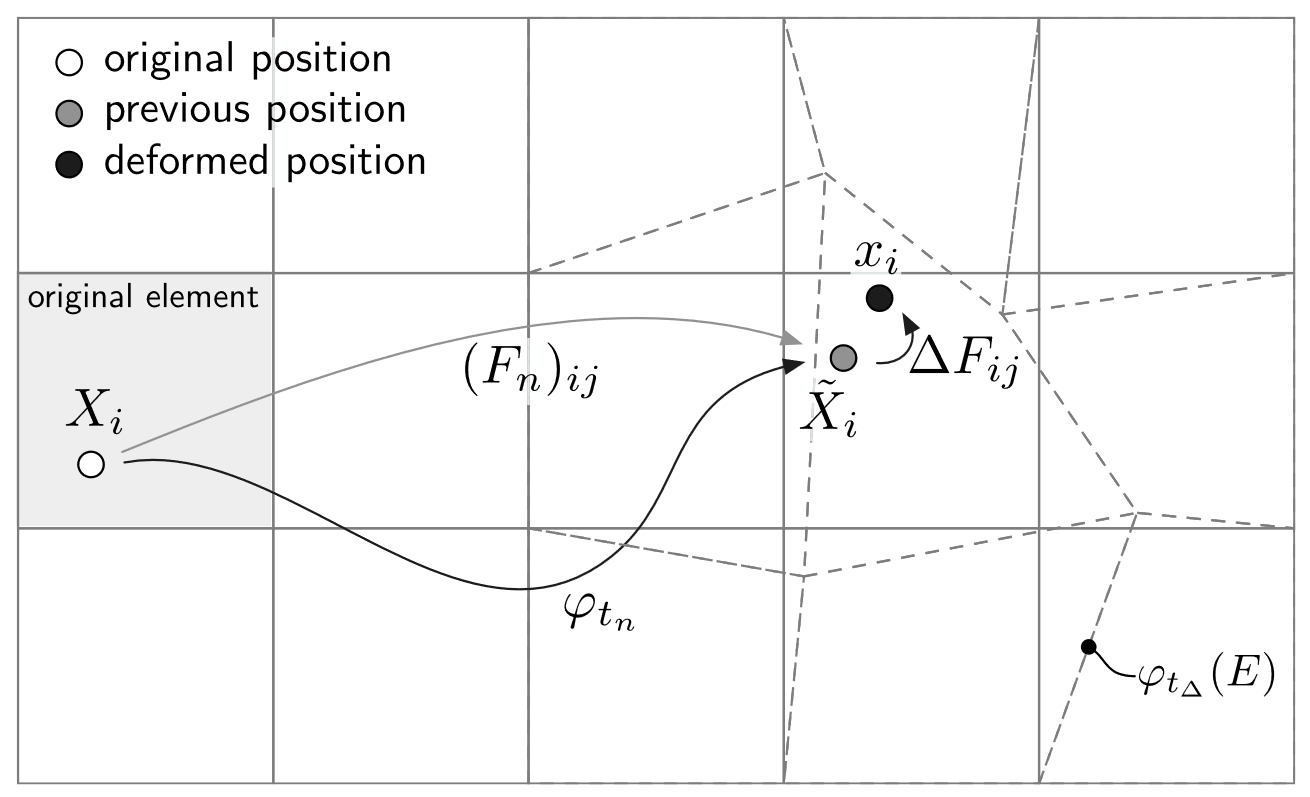
../../../_images/mpm-coombs.png — Fig. 8 Motion and deformation of a material point from the reference frame to the current configuration with a discretized mesh.¶

../../../_images/mpm-general-motion3D-light.svg — Fig. 9 Initial (undeformed), converged and current (deformed) configurations of a continuum body.¶

../../../_images/mpm-general-motion3D-dark.svg

Referring to Fig. 9, we use the following equations for mapping between initial, converged and current configurations.

\[ \begin{aligned} \bm{F} &= \bm{\tilde{F}} \bm{F}_n, \quad J = \tilde{J} J_n, \\ J &= \frac{d\text{v}}{dV}, \quad \tilde{J} = \frac{d\text{v}}{d\tilde{V}}, \quad J_n = \frac{d\tilde{V}}{dV}, \\ \bm{u} &= \bm{x} - \bm{X}, \quad \bm{\tilde{u}} = \bm{x} - \bm{\tilde{X}}, \quad \bm{u}_n = \bm{\tilde{X}} - \bm{X}, \\ \left(\nabla_x \diff \bm{u} \right)^T \tilde{\bm F}^{-T} &= \left(\nabla_{\tilde X} \diff \bm{u} \tilde{\bm F}^{-1} \right)^T \tilde{\bm F}^{-T} = \left(\tilde{\bm F}^{-1} \diff \tilde{\bm F} \tilde{\bm F}^{-1} \right)^{T} = -\diff \tilde{\bm F}^{-T}. \end{aligned} \]

In current configuration, our residual is computed with respect to \(\Omega_0\). However, for updated Lagrangian formulation we need to compute our integral with respect o previous converged configuration \(\Omega_{n} = \tilde{\Omega}\). We have

(326)¶\[ \int_{\Omega_{0}} \nabla_{x} \bm{v} \tcolon \bm{\tau} \, dV = \int_{\Omega_{0}} \nabla_{\tilde{X}} \bm{v} \tilde{\bm F}^{-1} \tcolon \bm{\tau} \, dV = \int_{\tilde{\Omega}} \nabla_{\tilde{X}} \bm{v} \tcolon \underbrace{\frac{1}{J_n}\bm{\tau} \tilde{\bm F}^{-T}}_{\tilde{\bm P}} \, d\tilde{V}. \]

In Jacobian we have

(327)¶\[ \begin{aligned} \int_{\Omega_{0}} \nabla_{x} \bm{v} \tcolon \left[\diff \bm{\tau} - \bm{\tau} \left(\nabla_x \diff \bm{u} \right)^T \right]\, dV &= \int_{\tilde{\Omega}} \nabla_{\tilde{X}} \bm{v} \tcolon \frac{1}{J_n} \left[ \diff \bm{\tau} - \bm{\tau} \left(\nabla_x \diff \bm{u} \right)^T \right] \tilde{\bm F}^{-T} \, d\tilde{V} \\ &= \int_{\tilde{\Omega}} \nabla_{\tilde{X}} \bm{v} \tcolon \underbrace{\frac{1}{J_n} \left[ \diff \bm{\tau} \tilde{\bm F}^{-T} + \bm{\tau} \diff \tilde{\bm F}^{-T} \right]}_{\diff \tilde{\bm{P}}}\, d\tilde{V} \end{aligned} \]

Note that (326) and (327) are written in the converged configuration. Using the deformation gradient \(\tilde{\bm F}\) and the relation \(d\tilde{V} = J_n dV\), we obtain a weak form similar to (104) in the current configuration as

(328)¶\[ r(\bm u) \coloneqq \int_{\tilde{\Omega}}{\nabla_x \bm{v} \tcolon \frac{1}{J_n} \bm{\tau}} \, d\tilde{V} - \int_{\tilde{\Omega}}{\bm{v} \cdot \frac{1}{J_n} \rho_0 \bm{g}} \, d\tilde{V} - \int_{\partial \tilde{\Omega}}{\bm{v} \cdot \bar{\bm t}} \, d\tilde{A} = 0, \quad \forall \bm{v} \in \mathcal{V}, \]

with Jacobian similar to (107) as

(329)¶\[ \int_{\tilde{\Omega}} \nabla_x \bm{v} \tcolon \frac{1}{J_n}\left( \diff \bm{\tau} - \bm{\tau} \left( \nabla_x \diff \bm{u} \right)^T \right) d\tilde{V} = -r(\bm u). \]

Therefore, for the MPM model in Ratel, all the weak forms and linearizations introduced in the current configuration for different material models remain valid, but the deformation gradient must be defined as \(\bm{F} = \tilde{\bm{F}} \bm{F}_n\).

Stabilization¶

It is often desirable to simulate a solid body composed of material points which does not fully or uniformly cover the background mesh. A common example of such a problem is the simulation of an elastic beam clamped on one end deforming under gravity, as shown in Fig. 10.

../../../_images/mpm-beam-light.svg — Fig. 10 Material point method simulation of the deflection of an elastic beam under self-weight; initial configuration (left), time \(t=0.3\) (right).¶

In the initial configuration, material points are placed uniformly in the top row of cells, while the remaining cells are empty. In practice, such a point distribution causes some numerical difficulty, but is possible to solve without additional stabilization. Once several time steps have passed, however, the points become distributed in a far more degenerate fashion; some cells contain only one or two material points. As such, the stiffness matrix for this system is both singular and, even if all zero singular values are removed via the SVD, the reduced system is very ill-conditioned.

Solving problems with under-populated cells requires the introduction of stabilization terms which produce a better conditioned stiffness matrix. Currently, Ratel implements one such stabilization method: background stiffness.

Background Stiffness Stabilization¶

Theory¶

This method introduces an artificial elasticity to the background mesh. Specifically, in addition to the terms in (328), the residual adds a term:

(330)¶\[ r_{\text{stab}}(\bm u) \coloneqq r(\bm u) + \int_{\tilde{\Omega}}{\nabla_x \bm{v} \tcolon \tilde{\bm{\tau}}}_{\text{stab}} \, \diff\tilde{V}, \]

where \(\tilde{\bm{\tau}}_{\text{stab}}\) is the Kirchhoff stress due to the incremental strain from the previously converged configuration to the current configuration. For a given constitutive model \(\bm\tau = \bm\tau(\bm e)\), the stabilization stress is defined as

(331)¶\[ \tilde{\bm{\tau}}_{\text{stab}} = \bm{\tau}(\tilde{\bm e}) = \bm{\tau}\left(\frac{1}{2}(\tilde{\bm F}^T \tilde{\bm{F}} - \bm{I})\right). \]

The Jacobian adds a similar term:

(332)¶\[ \begin{aligned} \int_{\tilde{\Omega}} \nabla_x \bm{v} &\tcolon \frac{1}{J_n}\left( \diff \bm{\tau} - \bm{\tau} \left( \nabla_x \diff \bm{u} \right)^T \right)\, \diff\tilde{V} \\ &+ \underbrace{\int_{\tilde{\Omega}} \nabla_x \bm{v} \tcolon \left( \diff \bm{\tau}_{\text{stab}} - \tilde{\bm{\tau}}_{\text{stab}} \left( \nabla_x \diff \bm{u} \right)^T \right)}_{\text{stabilization term}} = -r_{\text{stab}}(\bm u) \, \diff\tilde{V}, \end{aligned} \]

Critically, the integral in (330) and the second integral in (332) are computed with finite element basis functions and Gauss quadrature, not the material points. As a result, this is equivalent to computing the stress using any of the existing FEM models with respect to the incremental displacement (as opposed to the total displacement).

Command-Line Interface¶

Below, Table 36 shows the command-line options for background stiffness MPM stabilization.

Table 36 MPM Background Stiffness Stabilization Options¶
Option	Description	Default Value
`-mpm_stabilization_type background_stiffness`	Required to activate background stiffness stabilization.
`-mpm_stabilization_background_stiffness_model`	Material model to use for background stiffness. This must be a FEM material with the same active field sizes as the active MPM material. Required.
`-mpm_stabilization_background_stiffness_[material options]`	Material options for the specified model. See Material Properties for more details.

Example¶

Initializing Material Properties¶

There are three ways to assign material properties to material points.

Conforming Mesh¶

The simplest approach simply uses the mesh regions of the background mesh in the initial configuration to assign material properties to points. As for FEM, define a material for each mesh region. Then, before the first timestep, each material point will have its local material properties set according to the mesh cell in which it is contained.

This initialization method is the easiest to use, but requires that a conformal hexahedral mesh of the desired geometry can be defined. Additionally, since the background mesh is used for both initialization and subsequent solves, any poorly shaped elements in the mesh due to the conforming geometry will negatively impact the numerical performance and accuracy of the solver.

Command-Line Interface¶

For completeness, Table 37 shows the command-line options for initializing material points in a conformal mesh. In addition to the MPM specific options, materials and mesh options should be specified in the same fashion as for FEM, see Command Line Options.

Table 37 MPM Initialization Options¶
Option	Description	Default Value
`-method mpm`	Required to enable MPM
`-mpm_point_location_type [uniform \| gauss \| random]`	Initial per-cell point distribution within each background mesh cell.	`uniform`
`-mpm_num_points_per_cell [int]`	Number of material points to place in each cell. For `uniform` or `gauss` point location type, this will be rounded to the nearest cube. Required.
`-mpm_projection [lumped \| consistent]`	Type of projection to use from swarm to mesh. Lumped retains monotonicity but consistent is generally more accurate. Consistent falls back to lumped if projection fails to converge. Lumped is highly recommended if some cells may have very few points.	`consistent`
`-mpm_output_fields_projection [lumped \| consistent]`	Type of mass projection to use from swarm to mesh for output fields. Lumped retains monotonicity but consistent is generally more accurate. Lumped is highly recommended if some cells may have very few points.	Value set to `-mpm_projection`
`-dm_plex_hash_location [bool]`	Enable spatial hashing for point location. This is highly recommended to improve performance.	`false`

Example¶

Material Mesh¶

Often, one may have a mesh with well-defined material regions for use with FEM which is not suitable for use as an MPM background mesh. For example, a tetrahedral mesh or a mesh with highly distorted elements. In this case, material properties can be assigned to material points based on a secondary material mesh. The material mesh can be defined using any format supported by the PETSc unstructured mesh DMPlex interface. This includes:

Simplex/tetrahedral meshes
Mixed topology meshes, such as hexahedral, pyramid, and simplex hybrid meshes
High-order geometry
Arbitrary number of volumetric mesh regions

Warning

Performance Implications of Using a Material Mesh

The material mesh initialization interface is very flexible, but can be extremely slow in certain circumstances. The implementation reads the material mesh, sets it as the background mesh for the DMSwarm, and then migrates the material points in order to find their location in the material mesh. If the background mesh and material mesh are distributed across processes differently, a large communication cost may be incurred. Then, each point has its material properties assigned using a loop on the CPU, which may also be expensive for large numbers of points. Finally, the background mesh is restored and points are migrated back to their original processes, incurring a similar communication overhead.

While these costs may seem quite dire, this procedure is performed only once per simulation. Amortized over the entire simulation, the initialization cost may be relatively minor.

Command-Line Interface¶

In order to use a material mesh, the option -mpm_initialization material_mesh must be provided. Additional options, including specification of material regions, are given in Table 38.

Table 38 MPM Material Mesh Options¶
Option	Description	Default Value
`-method mpm`	Required to enable MPM
`-mpm_point_location_type [uniform \| gauss \| random]`	Initial per-cell point distribution within each background mesh cell.	`uniform`
`-mpm_num_points_per_cell [int]`	Number of material points to place in each cell. For `uniform` or `gauss` point location type, this will be rounded to the nearest cube. Required.
`-mpm_projection [lumped \| consistent]`	Type of projection to use from swarm to mesh. Lumped retains monotonicity but consistent is generally more accurate. Consistent falls back to lumped if projection fails to converge. Lumped is highly recommended if some cells may have very few points.	`consistent`
`-mpm_output_fields_projection [lumped \| consistent]`	Type of mass projection to use from swarm to mesh for output fields. Lumped retains monotonicity but consistent is generally more accurate. Lumped is highly recommended if some cells may have very few points.	Value set to `-mpm_projection`
`-dm_plex_hash_location [bool]`	Enable spatial hashing for point location. This is highly recommended to improve performance.	`false`
`-mpm_initialization material_mesh`	Required to enable the use of a material mesh.
`-mpm_material_mesh_dm_plex_filename [path to material mesh]`	Path to material mesh file.
`-mpm_material_mesh_dm_plex_hash_location`	Enable spatial hashing for point location. This is highly recommended to improve performance.
`-mpm_material_mesh_[dm options]`	Any valid option for the PETSc `DM` or `DMPlex` objects can be used to specify the material mesh.
`-mpm_material [string list]`	List of names to use as labels for each material. If not provided, a single material is assumed and can be specified with the prefix `-mpm_[material options]`.
`-mpm_[material name]_model`	Material to use (`elasticity-mpm-neo-hookean-current`, `elasticity-mpm-neo-hookean-damage-current`) for a given material. This model must be the same as the model used for the background mesh and all other materials. Required.
`-mpm_[material name]_label_name [str]`	Domain label in the material mesh specifying the type of volume to use for specifying materials.	`"Cell Sets"`
`-mpm_[material name]_label_value [int]`	Domain value in the material mesh specifying the volume to use for a given material.	`1`
`-mpm_[material name]_skip_checks [bool]`	If `true`, material property checks will be skipped and no state will be retained by points of this material. Useful, e.g., for “sticky air”.	`false`
`-mpm_[material name]_[material options]`	Material options for the specified model. See Material Properties for more details.

The background mesh is specified via the typical -dm_* options. It is often favorable to choose a background mesh which is either regular or close to regular to improve solver performance and accuracy.

In addition to defining the materials for the material mesh, a “dummy” material must also be defined for the background mesh. The dummy material requires that the following is set:

The -model for the material should be the same as the model used for the material mesh.
Any global options (mainly -use_AT1 and -use_offdiagonal for the elasticity-mpm-neo-hookean-damage-current model) should be set on the background mesh. Values provided to the material mesh materials will be ignored.

Additional material properties on the background mesh material will be ignored, and input validation on these properties can be skipped via the -skip_checks flag.

See the below example for more details.

Example¶

Voxel Data¶

The voxel interface provides a compromise between the simplicity of the conformal mesh and the flexibility of the material mesh. This interface allows material label values to be assigned to points based on a regular grid of cubes. Each cube has the same side length \(s\), specified with -mpm_voxel_pixel_size, and the entire voxel data is assumed to cover the domain \([0,n_x \cdot s] \times [0,n_y \cdot s] \times [0,n_z \cdot s]\).

The voxel data is specified via -mpm_voxel_filename [path], which should be a file in the format:

DIM N_X N_Y N_Z

VALUE_X1_Y1_Z1 VALUE_X1_Y1_Z2 ... VALUE_X1_Y1_Z(N_Z)
VALUE_X1_Y2_Z1 VALUE_X1_Y2_Z2 ... VALUE_X1_Y2_Z(N_Z)
...
VALUE_X1_Y(N_Y)_Z1 VALUE_X1_Y(N_Y)_Z2 ... VALUE_X1_Y(N_Y)_Z(N_Z)

VALUE_X2_Y1_Z1 VALUE_X2_Y1_Z2 ... VALUE_X2_Y1_Z(N_Z)
VALUE_X2_Y2_Z1 VALUE_X2_Y2_Z2 ... VALUE_X2_Y2_Z(N_Z)
...
VALUE_X2_Y(N_Y)_Z1 VALUE_X2_Y(N_Y)_Z2 ... VALUE_X2_Y(N_Y)_Z(N_Z)

...

VALUE_X(N_X)_Y1_Z1 VALUE_X(N_X)_Y1_Z2 ... VALUE_X(N_X)_Y1_Z(N_Z)
VALUE_X(N_X)_Y2_Z1 VALUE_X(N_X)_Y2_Z2 ... VALUE_X(N_X)_Y2_Z(N_Z)
...
VALUE_X(N_X)_Y(N_Y)_Z1 VALUE_X(N_X)_Y(N_Y)_Z2 ... VALUE_X(N_X)_Y(N_Y)_Z(N_Z)

Extra whitespace in the voxel data is ignored to allow for human-readable formatting of small voxel data files. Each VALUE_X(i)_Y(j)_Z(k) is an integer value corresponding to the -mpm_[material name]_label_value of the material for that voxel. If a value does not have a corresponding material, it is automatically removed from the simulation. This allows for the embedding of more complex structures which are surrounded by void.

The primary use of the voxel data interface is to read voxelized and segmented data which has been assigned a numerical index based on its material. For a grayscale TIFF stack, the corresponding Ratel voxel data can be generated using Script to convert a TIFF stack into voxel data which can be read by Ratel and the numpy and tifffile packages.

Listing 1 Script to convert a TIFF stack into voxel data which can be read by Ratel¶

import numpy as np
from tifffile import TiffFile, TiffSequence
from pathlib import Path

def load_tiff_stack(tiffstack: Path) -> np.ndarray:
    """
    Load a stack of TIFF files into a 3D numpy array.
    """
    # Load the voxel data
    if tiffstack.is_dir():
        # If the input is a directory, load all TIFF files in the directory
        with TiffSequence(f'{Path(tiffstack) / "*.tif"}') as tif:
            # Read all images
            voxel_data = tif.asarray()
    else:
        with TiffFile(tiffstack) as tif:
            voxel_data = tif.asarray()

    # Move the axes to (x, y, z) format
    voxel_data = np.moveaxis(voxel_data, [0, 1, 2], [2, 1, 0])
    return voxel_data

def dump(dst: Path, voxel_data: np.ndarray, keep_grain_ids: bool = False) -> None:
    """
    Dump the tiff stack array to a file.
    """
    if not keep_grain_ids:
        # Remove the grain IDs from the voxel data
        voxel_data[voxel_data >= 2] = 2
    # Save the voxel data to a file
    np.savetxt(dst, voxel_data.flatten().reshape((1, voxel_data.size)),
               header=f'{len(voxel_data.shape)} ' + ' '.join(map(str, voxel_data.shape)),
               fmt='%d', delimiter=' ', comments='')

if __name__ == '__main__':
    tiff_file = Path("/path/to/tif/stack")
    output_file = Path("/path/to/output.dat")
    data = load_tiff_stack(tiff_file)
    dump(output_file, data)

Command-Line Interface¶

The -mpm_initialization voxel option is required to enable voxel data material point initialization. See Table 39 for a full list of options.

Table 39 MPM Voxel Options¶
Option	Description	Default Value
`-method mpm`	Required to enable MPM
`-mpm_point_location_type [uniform \| gauss \| random]`	Initial per-cell point distribution within each background mesh cell.	`uniform`
`-mpm_num_points_per_cell [int]`	Number of material points to place in each cell. For `uniform` or `gauss` point location type, this will be rounded to the nearest cube. Required
`-mpm_projection [lumped \| consistent]`	Type of projection to use from swarm to mesh. Lumped retains monotonicity but consistent is generally more accurate. Consistent falls back to lumped if projection fails to converge. Lumped is highly recommended if some cells may have very few points.	`consistent`
`-mpm_output_fields_projection [lumped \| consistent]`	Type of mass projection to use from swarm to mesh for output fields. Lumped retains monotonicity but consistent is generally more accurate. Lumped is highly recommended if some cells may have very few points.	Value set to `-mpm_projection`
`-dm_plex_hash_location [bool]`	Enable spatial hashing for point location. This is highly recommended to improve performance.	`false`
`-mpm_initialization voxel`	Required to enable the use of a voxel data.
`-mpm_voxel_pixel_size [double]`	Side length of each voxel cube. Required.
`-mpm_voxel_filename [path]`	Path to voxel data file. Required.
`-mpm_material [string list]`	List of names to use as labels for each material. If not provided, a single material is assumed and can be specified with the prefix `-mpm_[material options]`.
`-mpm_[material name]_model`	Material to use (`elasticity-mpm-neo-hookean-current`, `elasticity-mpm-neo-hookean-damage-current`) for a given material. This model must be the same as the model used for the background mesh and all other materials. Required.
`-mpm_[material name]_label_value [int]`	Voxel value for which this material should be used.	`1`
`-mpm_[material name]_skip_checks [bool]`	If `true`, material property checks will be skipped and no state will be retained by points of this material. Useful, e.g., for “sticky air”.	`false`
`-mpm_[material name]_[material options]`	Material options for the specified model. See Material Properties for more details.

Similar to the material mesh interface, the voxel interface requires that a “dummy” material also be defined for the background mesh. The dummy material requires that the following is set:

The -model for the material should be the same as the model used for the material mesh.
Any global options (mainly -use_AT1 and -use_offdiagonal for the elasticity-mpm-neo-hookean-damage-current model) should be set on the background mesh. Values provided to the material mesh materials will be ignored.

Additional material properties on the background mesh material will be ignored, and input validation on these properties can be skipped via the -skip_checks flag.

LAMMPS Output Data¶

Point fields can also be initialized from the output dump files from LAMMPS. This interface allows material label values to be assigned to points based on a collection of spheres. The coordinates and radii of spheres can be uniformly rescaled via the -mpm_lammps_length_scale option.

The voxel data is specified via -mpm_lammps_filename [path], which should be a file in the format:

ITEM: NUMBER OF ATOMS
INT
ITEM: ATOMS id mol type radius x y z c_nb_peratom
INT INT INT REAL REAL REAL REAL INT
...

Note, LAMMPS output files include other ITEM tags, but these are the only ones utilized by Ratel; others will be ignored. The type, radius, and x, y, z coordinates are the only columns used by Ratel. The type should correspond to material label values specified as -mpm_[material name]_label_value. The label_value of 0 is reserved for a fallback material for any points not located in the sphere. If no fallback material is provided, such points will be removed.

Command-Line Interface¶

The -mpm_initialization lammps option is required to enable LAMMPS output-based material point initialization. See Table 40 for a full list of options.

Table 40 MPM LAMMPS Initialization Options¶
Option	Description	Default Value
`-method mpm`	Required to enable MPM
`-mpm_point_location_type [uniform \| gauss \| random]`	Initial per-cell point distribution within each background mesh cell.	`uniform`
`-mpm_num_points_per_cell [int]`	Number of material points to place in each cell. For `uniform` or `gauss` point location type, this will be rounded to the nearest cube. Required
`-mpm_projection [lumped \| consistent]`	Type of projection to use from swarm to mesh. Lumped retains monotonicity but consistent is generally more accurate. Consistent falls back to lumped if projection fails to converge. Lumped is highly recommended if some cells may have very few points.	`consistent`
`-mpm_output_fields_projection [lumped \| consistent]`	Type of mass projection to use from swarm to mesh for output fields. Lumped retains monotonicity but consistent is generally more accurate. Lumped is highly recommended if some cells may have very few points.	Value set to `-mpm_projection`
`-dm_plex_hash_location [bool]`	Enable spatial hashing for point location. This is highly recommended to improve performance.	`false`
`-mpm_initialization lammps`	Required to enable the use of LAMMPS output data.
`-mpm_lammps_length_scale [double]`	Scalar value applied to coordinates and radii. Optional.	`1.0`
`-mpm_lammps_filename [path]`	Path to LAMMPS output data file. Required.
`-material [string list]`	List of names to use as labels for each material. If not provided, a single material is assumed and can be specified with the prefix `-mpm_[material options]`.
`-mpm_[material name]_model`	Material to use (`elasticity-mpm-neo-hookean-current`, `elasticity-mpm-neo-hookean-damage-current`) for a given material. This model must be the same as the model used for the background mesh and all other materials. Required.
`-mpm_[material name]_label_value [int]`	Atom type value for which this material should be used.	`1`
`-mpm_[material name]_skip_checks [bool]`	If `true`, material property checks will be skipped and no state will be retained by points of this material. Useful, e.g., for “sticky air”.	`false`
`-mpm_[material name]_[material options]`	Material options for the specified model. See Material Properties for more details.

Similar to the material mesh interface, the LAMMPS interface requires that a “dummy” material also be defined for the background mesh. The dummy material requires that the following is set:

The -model for the material should be the same as the model used for the material mesh.
Any global options (mainly -use_AT1 and -use_offdiagonal for the elasticity-mpm-neo-hookean-damage-current model) should be set on the background mesh. Values provided to the material mesh materials will be ignored.

Additional material properties on the background mesh material will be ignored, and input validation on these properties can be skipped via the -skip_checks flag.

Example¶

Example - Initialization from LAMMPS Data

An example of initialization from LAMMPS data can be run with the command

$ ./bin/ratel-quasistatic examples/ymls/ex02-quasistatic-elasticity-mpm-neo-hookean-damage-current-lammps.yml

This example simulates the same problem as the material mesh example above: a multi-material model with a cylindrical rod embedded in a binder. The binder and rod are defined using a LAMMPS data file, with corresponding labels of 1 and 2, respectively.

ITEM: TIMESTEP
9561125
ITEM: NUMBER OF ATOMS
18
ITEM: BOX BOUNDS ff ff ss
0 10
0 10
0 2.5
ITEM: ATOMS id mol type radius x y z c_nb_peratom
100001 10145 1 5 1.0 1.0 0.0 1
100002 10145 1 5 5.0 0.0 0.0 1
100003 10145 1 5 9.0 1.0 0.0 1
100004 10145 1 5 0.0 5.0 0.0 1
100005 10145 2 5 5.0 5.0 0.0 1
100006 10145 1 5 10. 5.0 0.0 1
100007 10145 1 5 1.0 9.0 0.0 1
100008 10145 1 5 5.0 10. 0.0 1
100009 10145 1 5 9.0 9.0 0.0 1
100010 10145 1 5 1.0 1.0 1.25 1
100011 10145 1 5 5.0 0.0 1.25 1
100012 10145 1 5 9.0 1.0 1.25 1
100013 10145 1 5 0.0 5.0 1.25 1
100014 10145 2 5 5.0 5.0 1.25 1
100015 10145 1 5 10. 5.0 1.25 1
100016 10145 1 5 1.0 9.0 1.25 1
100017 10145 1 5 5.0 10. 1.25 1
100018 10145 1 5 9.0 9.0 1.25 1
100019 10145 1 5 1.0 1.0 2.5 1
100020 10145 1 5 5.0 0.0 2.5 1
100021 10145 1 5 9.0 1.0 2.5 1
100022 10145 1 5 0.0 5.0 2.5 1
100023 10145 2 5 5.0 5.0 2.5 1
100024 10145 1 5 10. 5.0 2.5 1
100025 10145 1 5 1.0 9.0 2.5 1
100026 10145 1 5 5.0 10. 2.5 1
100027 10145 1 5 9.0 9.0 2.5 1

The background mesh is an affine hexahedral mesh with the same dimensions as the material mesh. The “dummy” material only sets the model and the global -use_AT1 option.

# Ratel problem specification
# Dynamic material point material assignment using LAMMPS data
# Neo-Hookean hyperelastic material at finite strain with damage, MPM

order: 1

method: mpm

mpm:
  point_location_type: uniform
  num_points_per_cell: 27
  initialization: lammps
  lammps:
    filename: examples/data/ex02-quasistatic-elasticity-mpm-neo-hookean-damage-current-lammps.dump
    length_scale: 1.0e-1
  material: rod,binder
  binder:
    model: elasticity-mpm-neo-hookean-damage-current
    rho: 1.5
    E: 2.8
    nu: 0.3
    fracture_toughness: 1
    characteristic_length: 1.2
    damage_scaling: 1
    residual_stiffness: 1e-4
    label:
      value: 1
  rod:
    model: elasticity-mpm-neo-hookean-damage-current
    rho: 1
    E: 1
    nu: 0.3
    fracture_toughness: 1.6
    characteristic_length: 0.5
    damage_scaling: 1
    residual_stiffness: 1e-4
    label:
      value: 2

dm_plex:
  dim: 3
  box_faces: 3,3,3
  box_upper: 1,1,0.25
  simplex: 0
  hash_location:

material: dummy
dummy:
  model: elasticity-mpm-neo-hookean-damage-current
  use_AT1: false
  skip_checks:

bc:
  slip: 1,2
  slip_1:
    components: 0,1,2
    translate: 0,0,0
  slip_2:
    components: 0,1,2
    translate: 0,0,-0.025

remap:
  direction: z
  scale: 0.9

expected_strain_energy: 3.854621043167e-03
max_output_fields:
  components: damage
expected_max_output_fields: 1.17588498465e-02

Command-Line Interface¶

For completeness, all options relevant to the material point method in Ratel are provided in Table 41. In addition to those listed here, options for boundary conditions, meshes, materials, and more should be specified; see Command Line Options.

Table 41 Material Point Method Options¶
Option	Description	Default Value
`-method mpm`	Required to enable MPM
`-mpm_point_location_type [uniform \| gauss \| random]`	Initial per-cell point distribution within each background mesh cell.	`uniform`
`-mpm_num_points_per_cell [int]`	Number of material points to place in each cell. For `uniform` or `gauss` point location type, this will be rounded to the nearest cube. Required.
`-mpm_projection [lumped \| consistent]`	Type of projection to use from swarm to mesh. Lumped retains monotonicity but consistent is generally more accurate. Consistent falls back to lumped if projection fails to converge. Lumped is highly recommended if some cells may have very few points.	`consistent`
`-mpm_projection_[KSP/PC options] [lumped \| consistent]`	Any valid KSP or PC options to control the behavior of the projection solver. Common options (and their defaults) are `ksp_type` (`cg`), `ksp_max_it` (`10000`), `ksp_rtol` (`1e-12`), `pc_type` (`jacobi`). Only used for `consistent` projection.
`-mpm_output_fields_projection [lumped \| consistent]`	Type of mass projection to use from swarm to mesh for output fields. Lumped retains monotonicity but consistent is generally more accurate. Lumped is highly recommended if some cells may have very few points.	Value set to `-mpm_projection`
`-dm_plex_hash_location [bool]`	Enable spatial hashing for point location. This is highly recommended to improve performance.	`false`
`-mpm_stabilization_type [none \| background_stiffness]`	Type of stabilization to use. See Stabilization for more details.
`-mpm_stabilization_background_stiffness_model`	Material model to use for background stiffness. This must be a FEM material with the same active field sizes as the active MPM material. Only for background stiffness stabilization. Required.
`-mpm_stabilization_background_stiffness_[material options]`	Material options for the specified model. See Material Properties for more details. Only for background stiffness stabilization. Required.
`-mpm_initialization [default \| material_mesh \| voxel \| lammps]`	Initialization method for material properties, see Initializing Material Properties for more details.	`default`
`-mpm_material_mesh_dm_plex_filename [path to material mesh]`	Path to material mesh file. Only for `material_mesh` initialization.
`-mpm_material_mesh_dm_plex_hash_location`	Enable spatial hashing for point location. This is highly recommended to improve performance. Only for `material_mesh` initialization.
`-mpm_material_mesh_[dm options]`	Any valid option for the PETSc `DM` or `DMPlex` objects can be used to specify the material mesh. Only for `material_mesh` initialization.
`-mpm_voxel_pixel_size [double]`	Side length of each voxel cube. Only for `voxel` initialization. Required.
`-mpm_voxel_filename [path]`	Path to voxel data file. Only for `voxel` initialization. Required.
`-mpm_lammps_length_scale [double]`	Scalar value applied to coordinates and radii. Only for `lammps` initialization. Optional.	`1.0`
`-mpm_lammps_filename [path]`	Path to LAMMPS output data file. Only for `lammps` initialization. Required.
`-mpm_material [string list]`	List of names to use as labels for each material. Only for non-`default` initialization. If not provided, a single material is assumed and can be specified with the prefix `-mpm_[material options]`.
`-mpm_[material name]_model`	Material to use (`elasticity-mpm-neo-hookean-current`, `elasticity-mpm-neo-hookean-damage-current`) for a given material. This model must be the same as the model used for the background mesh and all other materials. Only for non-`default` initialization. Required.
`-mpm_[material name]_label_value [int]`	Value for which this material should be used. Meaning of “value” depends on initialization type. Only for non-`default` initialization.	`1`
`-mpm_[material name]_skip_checks [bool]`	If `true`, material property checks will be skipped and no state will be retained by points of this material. Useful, e.g., for “sticky air”. Only for non-`default` initialization.	`false`
`-mpm_[material name]_[material options]`	Material options for the specified model. Only for non-`default` initialization. See Material Properties for more details.